|
5/4/2017 0 Comments Image Based Lighting
Image Based Lighting (aka, IBL) is a 3D rendering technique which involves capturing an omnidirectional representation of real-world light information as an image, typically using a specialized camera. This image is then projected onto a dome or sphere analogously to environment mapping, and this is used to simulate the lighting for the objects in the scene. This allows highly detailed real-world lighting to be used to light a scene, instead of trying to accurately model illumination using an existing rendering technique. IBL often uses High Dynamic Range (aka, HDR) imaging for greater realism. This technique used in movies, games, and wide range of area which requires to render realistic scenes in real time. My Implementation Since IBL requires physically based lighting calculation, there are two big terms you need to implement. The diffuse term and the specular term. In this project, I used two different texture maps. One is Irradiance map for diffuse calculation(right image below), and the other is HDR map for specular calculation(left image below). You can use pre-calculated irradiance map or generate the map for yourself. 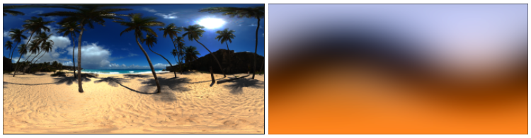 Lighting |

 |  |
 |  |
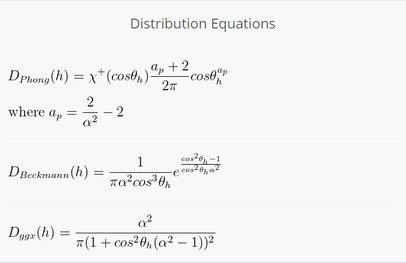 |  |
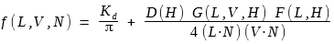
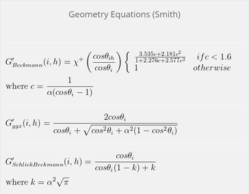
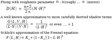
Pick each terms as one of these equations. In my case, I picked phong distribution, Schlick's fresnel equation, and approximation of geometric term :
Tone Mapping and Linear Color space
Before you start the calculation there is one thing you need to know. Since HDR images can contain colors in the range [0, Infinite], you need to convert this into the displayable range [0, 1]. An easy global tone-mapping calculation is :
Before you start the calculation there is one thing you need to know. Since HDR images can contain colors in the range [0, Infinite], you need to convert this into the displayable range [0, 1]. An easy global tone-mapping calculation is :
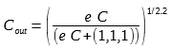
where 'e' is a total exposure control (in the range [0.1, 10000] for various of my test), and the exponent does the conversion from linear to gamma color space for final display.
Color Spaces
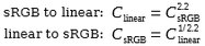
All lighting & color calculation should take place in linear color space while most input images and all output devices expect values in a non-linear color space (e.g. gamma color space or sRGB color space) Color values should be convverted from sRGB to linear on input and back to sRGB before output to the display device. The conversion can be calculated as :
Color Spaces
All lighting & color calculation should take place in linear color space while most input images and all output devices expect values in a non-linear color space (e.g. gamma color space or sRGB color space) Color values should be convverted from sRGB to linear on input and back to sRGB before output to the display device. The conversion can be calculated as :
Diffuse Calculation
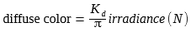
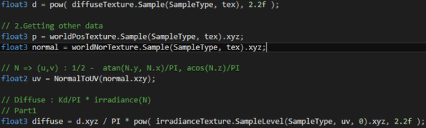
Step 1. Power the diffuse by 2.2f to convert the value from sRGB to linear space.
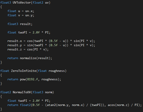
Step 2. Get a correct texture coordinate corresponding to object’s normal. (u,v) : 1/2 - atan(N.y, N.x)/PI, acos(N.z)/PI. I made this as a helper function called NormalToUV.
Step 3. Multiply diffuse / 2*PI with irradiance linear space color.
Step 2. Get a correct texture coordinate corresponding to object’s normal. (u,v) : 1/2 - atan(N.y, N.x)/PI, acos(N.z)/PI. I made this as a helper function called NormalToUV.
Step 3. Multiply diffuse / 2*PI with irradiance linear space color.
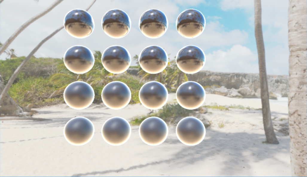
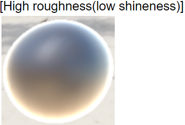
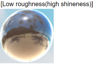
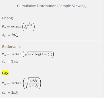
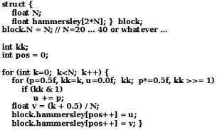
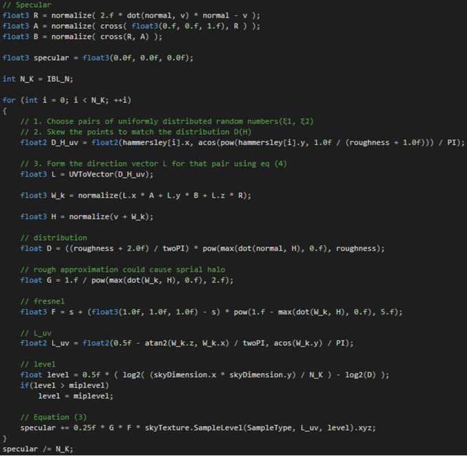
Unlike Diffuse term, Specular term calculation is much more complicated. There are two things you need to prepare before starting. First, convert roughness from [0...1] range to [0...infinity] range. This will be done by ZeroToInfinite function. Second, we need a way to choose N pairs of uniformly distributed random numbers. In this project, we used hammersley algorithm.(N means how many times will you sample)
Specular Calculation
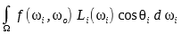
The specular portion of the lighting requires an approximation of the lighting integral where the function f(...) is specular portion of BRDF
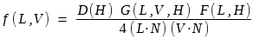
The Monte-Carlo approximation to this integral is
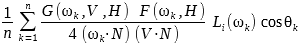
where the N directions W_k are chosen with probability p(W_k). If we choose p(W_k) = D(H) to cancel each other out, we can get this approximated equation above.
Helper Function
0 Comments
5/2/2017 0 Comments
Hatch Shading
 |  |
Hatching is a common technique used in Non-Photorealistic Rendering(NPR). For hatching, series of strokes are combined into textures. These compositions of strokes can convey the surface form through stroke orientation, the surface material through stroke arrangement and style, and the effect of light on the surface through stroke density.\
For hatching, strokes have to be chosen from a collection of possible strokes to convey some tonal value. This collections of strokes are called Prioritized Stroke Texture, and different mipmap levels can be precomputed and blended at run-time according to the given tonal value. To maintain a constant stroke width in screen space, the mipmap levels contain strokes of the same texel width. Thus, higher mipmap level contain fewer strokes than lower mipmap levels for representing the same tonal value.
Tonal Art Maps
In photorealistic rendering, the traditional approach for rendering complex detail is to capture it in the form of texture map. We apply this same approach to the rendering of hatching strokes for NPR. Strokes are pre-rendered into a set of texture images, and at runtime, the surface is rendered by appropriately blending these textures. To render a surface, we compute its desired tone value, and render the surface unlit using the texture of the appropriate tone. By selecting multiple textures on each face and blending them together, we can achieve fine local control over surface tone while at the same time maintaining spatial and temporal coherence of the stroke detail.
Another difficulty in applying conventional texture maps to NPR detail is that scaling does not achieve the desired effect. When magnifying an object, we would like to see more strokes appear, whereas ordinary texture mapping simply makes existing strokes larger. So we design the mipmap levels such that strokes have the same width in all levels. Finer levels maintain constant tone by adding new strokes to fill the enlarged gaps between the old strokes. This mipmap construction for the stroke image associated with each tone. We call the resulting sequence of mpmapped images a Tonal Art Map.(TAM)
Tonal Art Map consists of 2D grid of images. Since we render the surface by blending between textures corresnponding to different tones and different resolutions, it is important that the textures have a high degree of coherence. Here is the example of Tonal Art Map.
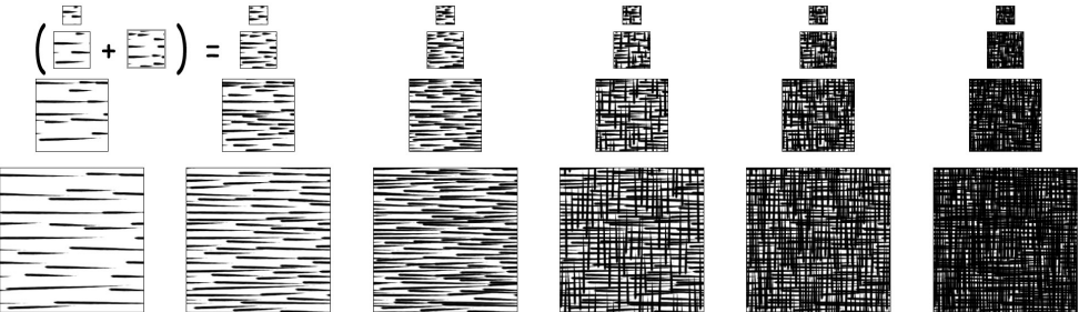
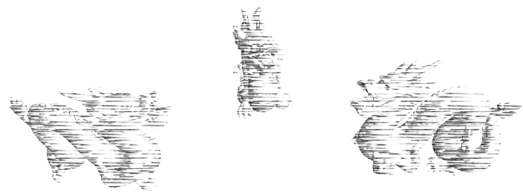
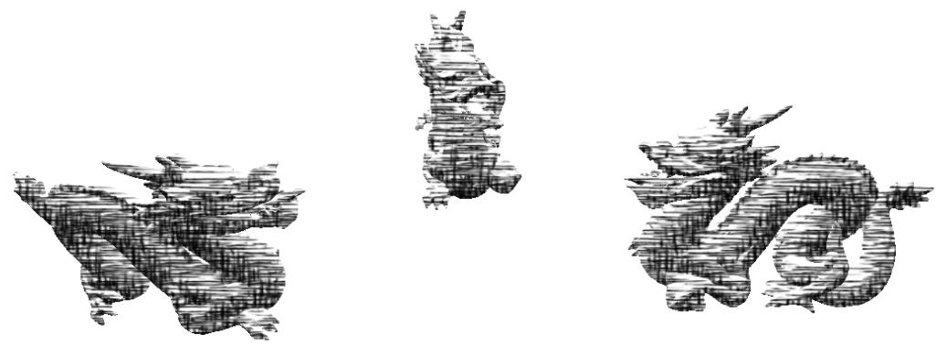
In this way of implementation, we need a number of textures based on how much detail you want to display. Since these series of textures only holds the image of strokes, we don't need their RGB values. Consider it as gray scaled image. In my implementation, I stored 6 textures into 2 textures. 1 map per each channel.
| As you can see, my implementation is quite simple. I used dot product of light vector and normal vector of the surface as its tonal value. Since I'm using 6 texture, I converted the result of dot product in range of [-1, 1] to range of [0,6]. This converted value 'Factor' will be used as blending weight of those textures. By doing this, I could determine how much strokes should be displayed on the surface based on the light position. Although this way of implementation highly rely on TAMs' image, the result could be different from what you've expected. In that case, you can try scaling the image to simply manipulate the width of strokes or replace the entire images as totally different one like below. 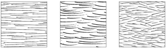 |  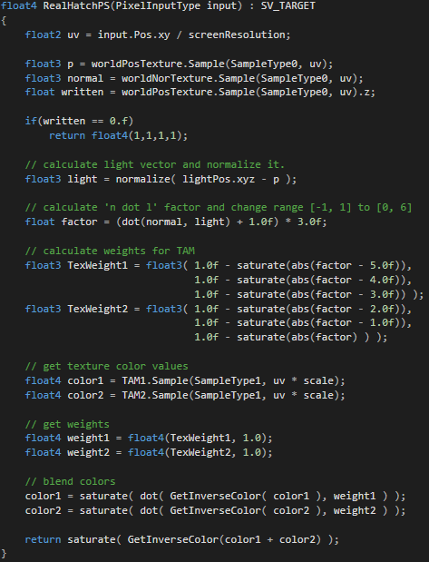 |
5/2/2017 0 Comments
Image Space Edge Detection


There are dozens of ways to detect and render edges in real-time. They all fit into roughly four categories: hardware, image-space, object-space, and miscellaneous methods. Hardware methods are quick and simple to implement, but with severe limitations. Image-space methods are a bit more involved and provide medium quality results. Object-space methods provide maximum quality and customizability, but often at the cost of speed. The miscellaneous category is a catch-all, but these methods tend to be quick and limited like hardware methods.
In this post, I'm going to explain about Sobel Edge Detection, one of the simplest way of creating nice edge around the object. All you need is the depth buffer.
For edge detection, image processing techniques typically apply convolutions to various properties of images or specialized images to generate gradients, a vector representing the local maximum change. In image processing, convolutions take the form of component-wise matrices called kernels or operators. These operators store numbers in each cell which are multiplied by some numerical property of the equivalent pixel in the input image. This operation is applied to every pixel in the input image, with optional special cases at the image borders where input data may not be available. The resulting output image data can be used in further calculations or displayed directly.
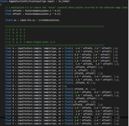
For each pixel (x) there are surrounding pixels (A, B, C, D, E, F, G, and H) except at the extreme borders of the viewport. The layout looks like below:
In this post, I'm going to explain about Sobel Edge Detection, one of the simplest way of creating nice edge around the object. All you need is the depth buffer.
For edge detection, image processing techniques typically apply convolutions to various properties of images or specialized images to generate gradients, a vector representing the local maximum change. In image processing, convolutions take the form of component-wise matrices called kernels or operators. These operators store numbers in each cell which are multiplied by some numerical property of the equivalent pixel in the input image. This operation is applied to every pixel in the input image, with optional special cases at the image borders where input data may not be available. The resulting output image data can be used in further calculations or displayed directly.
For each pixel (x) there are surrounding pixels (A, B, C, D, E, F, G, and H) except at the extreme borders of the viewport. The layout looks like below:
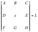
L represents the input pixels that will be used in conjunction with a kernel. Since a pixel is typically made up of color and alpha transparency information, the user must decide what property of the input image pixels he will use. You can use this operator wherever you can. But in this example, I used Depth Buffer as I mentioned above because depth shows the most trustworthy output. Sobel operator can have various dimension. 3x3, 5x5, 7x7 whaever.
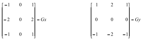
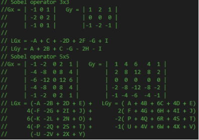
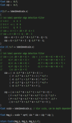
By multiplying this operator to the target pixel and pixels around the target pixel component-wisely, you will be able to get the direction of the gradient. LGx, LGy. But to detect the edge, you need the magnitude of the gradient.
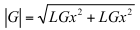
The gradient magnitude can be used directly in edge detection. By drawing black pixels where the gradient magnitude is greater than or less than a user-defined value, edges will be rendered. The process of choosing which pixels to draw based on the gradient (or any value) is called thresholding. I'll also post my implementation below. It is extremely easy to follow.
 |  |
